Using GAP on validation data

In this tutorial you will learn to use the trained ml potential on validation data. We do this to evaluate how well GAP has learned the energies and forces Let us start by importing some Python modules.

# uncomment the following line when running a jupyter notebook
# % matplot inline
import numpy as np
import matplotlib.pyplot as plt
import matplotlib
import ase
import ase.io
from ase import Atoms
from quippy.potential import Potential
from pathlib import Path

matplotlib.use("agg")

Then we define our project path. Replace the path with your own project path

PROJECT_PATH=Path("../../../solutions/")
CUT_OFF_FOLDER = PROJECT_PATH / "gap/cut_off_4A"

Then we load our ML potential.

ml_potential = Potential(param_filename=str(CUT_OFF_FOLDER / "SOAP.xml"))

Let us try out the ML potential. First, we create an Atoms object

distance = 3.3 # angstrom
two_argon_atoms = Atoms("Ar2", [[0, 0, 0], [0, 0, distance]])
two_argon_atoms.center(vacuum=3)
two_argon_atoms.pbc = [1, 1, 1]

Then we set the calculator to ml_potential and caculate the energy of the system

two_argon_atoms.set_calculator(ml_potential)
E = two_argon_atoms.get_potential_energy()
print(E)

/work/amam/ckf7015/fachlabor-dft-ml/tutorials/source/examples/plot_gap.py:45: FutureWarning: Please use atoms.calc = calc
  two_argon_atoms.set_calculator(ml_potential)
-1146.9424359067043

To evaluate the ML potential, we will compare predicted energies (and forces) with DFT energies (and forces). To do so, we will load the coordinates, energies and forces from the DFT simulation. Then we will predict the energy for the coordinates using the ML potential, and compare with the reference energies from the DFT simulation.

To quantify the error, we calculate the root mean square (RMS) error between the reference data and the predicted data.

def rms_dict(x_ref, x_pred):
    """ Takes two datasets of the same shape and returns a dictionary containing RMS error data"""

    x_ref = np.array(x_ref)
    x_pred = np.array(x_pred)

    if np.shape(x_pred) != np.shape(x_ref):
        raise ValueError('WARNING: not matching shapes in rms')

    error_2 = (x_ref - x_pred) ** 2

    average = np.sqrt(np.average(error_2))
    print(average)
    std_ = np.sqrt(np.var(error_2))

    return {'rmse': average, 'std': std_}

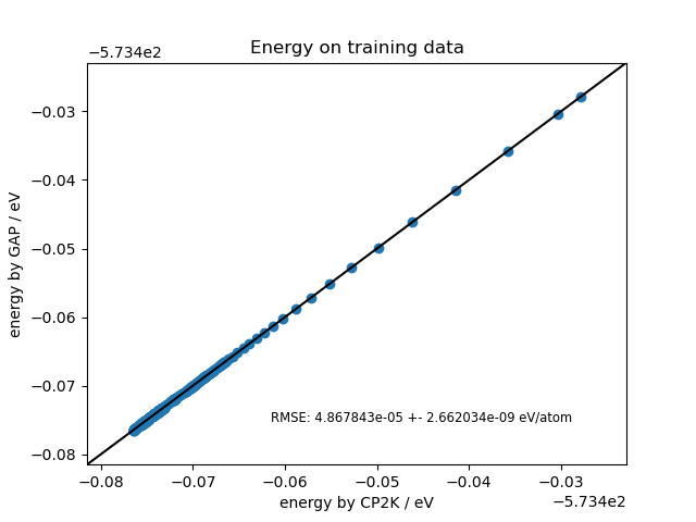
Next, we have a function to plot the predicted energy against the reference energy.

def energy_plot(in_file, ax, title='Plot of energy'):
    """ Plots the distribution of energy per atom on the output vs the input"""
    # read files
    in_frames = ase.io.read(in_file, ':')

    print(in_frames[0])
    print(f"number of frames {len(in_frames)}")
    print(f"position array has shape {in_frames[0].positions.shape}")
    print(f"{len(in_frames[0].get_chemical_symbols())}")
    # get reference potential energies calculated by DFT
    ener_in = [frame.get_potential_energy() / len(frame.get_chemical_symbols()) for frame in in_frames]
    ener_out = []
    # predict the energies using GAP.
    # set our ase calculator to ml_potential and then calculate the energy using that calculator.
    for frame in  in_frames:
        frame.set_calculator(ml_potential)
        ener_out+=[frame.get_potential_energy() / len(frame.get_chemical_symbols())]
    # make a scatter plot of the data
    ax.scatter(ener_in, ener_out)
    # get the appropriate limits for the plot
    for_limits = np.array(ener_in +ener_out)
    elim = (for_limits.min() - 0.005, for_limits.max() + 0.005)
    ax.set_xlim(elim)
    ax.set_ylim(elim)
    # add line of slope 1 for refrence
    ax.plot(elim, elim, c='k')
    # set labels
    ax.set_ylabel('energy by GAP / eV')
    ax.set_xlabel('energy by CP2K / eV')
    #set title
    ax.set_title(title)
    # add text about RMSE
    _rms = rms_dict(ener_in, ener_out)
    rmse_text = 'RMSE:\n' + str(np.round(_rms['rmse'], 5)) + ' +- ' + str(np.round(_rms['std'], 5)) + 'eV/atom'
    rmse_text = f"RMSE: {_rms['rmse']:2e} +- {_rms['std']:2e} eV/atom"
    ax.text(0.9, 0.1, rmse_text, transform=ax.transAxes, fontsize='small', horizontalalignment='right',
            verticalalignment='bottom')

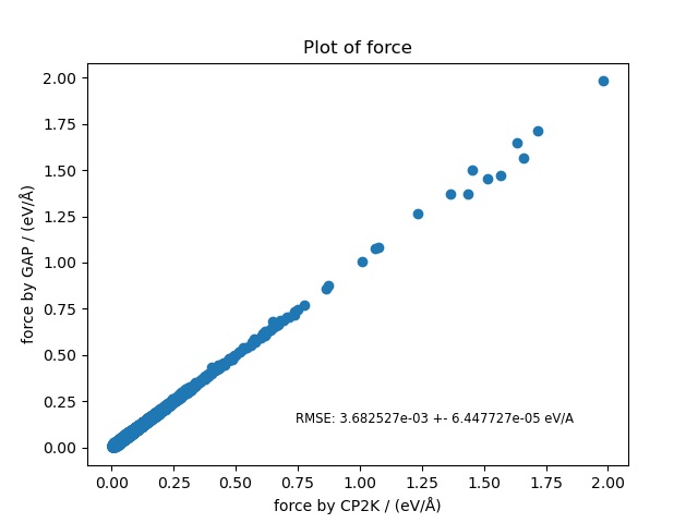
Then, we have a function to plot the predicted force against the reference force.

def force_plot(in_file, ax, symbol='HO', title='Plot of force'):
    """ Plots the distribution of force components per atom on the output vs the input
        only plots for the given atom type(s)"""

    in_atoms = ase.io.read(in_file, ':')

    symbol=["Ar"]
    # extract data for only one species
    in_force, out_force = [], []
    for at_in in in_atoms:
        # get the symbols
        sym_all = at_in.get_chemical_symbols()
        # add force for each atom
        for j, sym in enumerate(sym_all):
            if sym in symbol:
                in_force.append(at_in.get_forces()[j])
        at_in.set_calculator(ml_potential)
        for j, sym in enumerate(sym_all):
            if sym in symbol:
                out_force.append(at_in.get_forces()[j])
    print(len(in_force))
    print(in_force[0].shape)
    # convert to np arrays, much easier to work with
    in_force = np.array(in_force)
    out_force = np.array(out_force)
    in_force = np.sqrt(np.sum(in_force**2, axis=1))
    out_force = np.sqrt(np.sum(out_force**2, axis=1))
    print(in_force.shape)
    # scatter plot of the data
    ax.scatter(in_force, out_force)
    # set labels
    ax.set_ylabel('force by GAP / (eV/Å)')
    ax.set_xlabel('force by CP2K / (eV/Å)')
    #set title
    ax.set_title(title)
    # add text about RMSE
    _rms = rms_dict(in_force, out_force)
    #rmse_text = 'RMSE:\n' + str(np.round(_rms['rmse'], 5)) + ' +- ' + str(np.round(_rms['std'], 5)) + 'eV/Å'
    rmse_text = f"RMSE: {_rms['rmse']:2e} +- {_rms['std']:2e} eV/A"
    ax.text(0.9, 0.1, rmse_text, transform=ax.transAxes, fontsize='small', horizontalalignment='right',
            verticalalignment='bottom')
    return _rms

Finally, we plot the error and force correlation plots for the training data.

fig, ax = plt.subplots(1, 1)
energy_plot(PROJECT_PATH / "gap/train.xyz", ax, "Energy on training data")
fig.savefig(CUT_OFF_FOLDER / "energy_plot_train.png")


fig, ax = plt.subplots(1, 1)
rmse = force_plot(PROJECT_PATH / "gap/train.xyz", ax, "Force on training data")
fig.savefig(CUT_OFF_FOLDER / "force_plot_train.png")
np.savetxt(CUT_OFF_FOLDER / "force_rmse_train.txt", [rmse["rmse"], rmse["std"]])

• 
• 

Atoms(symbols='Ar108', pbc=True, cell=[17.0742, 17.0742, 17.0742], calculator=SinglePointCalculator(...))
number of frames 500
position array has shape (108, 3)
108
/work/amam/ckf7015/fachlabor-dft-ml/tutorials/source/examples/plot_gap.py:88: FutureWarning: Please use atoms.calc = calc
  frame.set_calculator(ml_potential)
4.8678426428232424e-05
/work/amam/ckf7015/fachlabor-dft-ml/tutorials/source/examples/plot_gap.py:129: FutureWarning: Please use atoms.calc = calc
  at_in.set_calculator(ml_potential)
54000
(3,)
(54000,)
0.00368252725422809

Plot force and error correlation for your validation data set as well.