Calculating the radial distribution function

In this tutorial we will learn how to analyse (ab-initio) molecular dynamics trajectories. We will use the tool MDAnalysis to read our simulation data files and calculate the radial distribution function.

Wikipedia page on RDF: MDAnalysis documentation on RDF:

We first import our python modules

import numpy as np
import matplotlib.pyplot as plt
from pathlib import Path

import MDAnalysis as mda
from MDAnalysis.analysis.rdf import InterRDF

Then we define our project path. Replace the path with your own project path

PROJECT_PATH=Path("../../../solutions/")

Next, we load our simulation output.

universe = mda.Universe(PROJECT_PATH / "dft"/ "Argon_Simulation-pos-1.xyz")

# The Universe object contains the atomic positions for each timestep. # Note that the xyz file does not contain any information on the dimensions

print(f"dimensions from xyz file {universe.dimensions}")

dimensions from xyz file None

So we must set the dimensions ourself to

box_l = 17.0742
universe.dimensions = [box_l, box_l, box_l, 90, 90, 90]

Let’s also check how many frames we’ve loaded with

print(f"loaded {len(universe.trajectory)} frames")

loaded 10001 frames

We now want to run an radial distribution analysis using InterRDF

rdf = InterRDF(universe.atoms, universe.atoms,
               n_bins = 100,
               range = (1.0, box_l / 2)
               )

We then run the analysis with

rdf.run()

/fibus/fs3/0b/ckf7015/.local/lib/python3.11/site-packages/MDAnalysis/analysis/base.py:522: UserWarning: Reader has no dt information, set to 1.0 ps
  self.times[idx] = ts.time

<MDAnalysis.analysis.rdf.InterRDF object at 0x7fee45ffb490>

Next, we plot our results

plt.plot(rdf.results.bins, rdf.results.rdf)
plt.xlabel("$r$ in A")
plt.ylabel("g(r)")

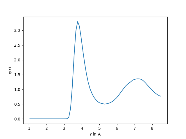
Text(42.597222222222214, 0.5, 'g(r)')

and save our figure

plt.savefig(PROJECT_PATH / "lammps" / "rdf.png", dpi=300)